Colors
Introduction
Script visuals play a crucial role in the usability of indicators written in Lipi Script. Well-designed plots and drawings make indicators more intuitive and easier to understand. Effective visual designs establish a hierarchy, ensuring that the most important information stands out, while less critical details remain unobtrusive.
Using colors in Lipi Script can be as simple or as complex as needed. With 4,294,967,296 possible color and transparency combinations, Lipi Script allows you to apply them to:
- Any plotted or drawn element in an indicator’s visual space, such as lines, fills, text, or candles.
- The background of a script’s visual space, whether in its own pane or overlaid on the chart.
- The bars or bodies of candles on the chart.
A script can only modify the visual elements it creates. The only exception is that pane indicators can color chart bars or candles.
Lipi Script provides built-in colors like color.green and functions like color.rgb() to dynamically generate any color within the RGBA color space.
Transparency
Each color in Lipi Script is defined by four components:
- Red, Green, and Blue (RGB): Values range from 0-255, as per the RGB color model.
- Transparency: Represented by values between 0-100, where:
0is fully opaque.100makes the color completely invisible. Transparency is often referred to as the Alpha channel (from the RGBA model). In functions, transparency can take “float” values, allowing finer control with 256 underlying alpha levels.
The transparency setting determines how opaque a color appears. Modulating transparency is vital for creating advanced visuals or layering colors, ensuring certain elements dominate or blend harmoniously.
Z-index
When elements are placed in a script’s visual space, they have a relative depth along the z-axis. The z-index determines their stacking order, with higher values appearing on top.
In Lipi Script, elements are grouped by their type, and each group has a fixed position on the z-axis. Within the same group, elements created later in the script logic appear above earlier ones. Elements from one group cannot move outside their designated z-index region. For example, a plot can never overlap a table because tables have the highest z-index.
Z-index Order (Low to High)
- Background colors
- Fills
- Plots
- Horizontal lines (Hlines)
- Line fills (LineFills)
- Lines
- Boxes
- Labels
- Tables
By using explicit_plot_zorder = true in indicator(), you can control the relative z-index of plot*(), hline(), and fill() visuals based on their sequential order in the script.
Constant Colors
Lipi Script includes 17 built-in colors. This table provides their names, hexadecimal equivalents, and RGB values as arguments for color.rgb():
| Name | Hex | RGB Values |
|---|---|---|
color.aqua | #00BCD4 | color.rgb(0, 188, 212) |
color.black | #363A45 | color.rgb(54, 58, 69) |
color.blue | #2196F3 | color.rgb(33, 150, 243) |
color.fuchsia | #E040FB | color.rgb(224, 64, 251) |
color.gray | #787B86 | color.rgb(120, 123, 134) |
color.green | #4CAF50 | color.rgb(76, 175, 80) |
color.lime | #00E676 | color.rgb(0, 230, 118) |
color.maroon | #880E4F | color.rgb(136, 14, 79) |
color.navy | #311B92 | color.rgb(49, 27, 146) |
color.olive | #808000 | color.rgb(128, 128, 0) |
color.orange | #FF9800 | color.rgb(255, 152, 0) |
color.purple | #9C27B0 | color.rgb(156, 39, 176) |
color.red | #F23645 | color.rgb(242, 54, 69) |
color.silver | #B2B5BE | color.rgb(178, 181, 190) |
color.teal | #089981 | color.rgb(8, 153, 129) |
color.white | #FFFFFF | color.rgb(255, 255, 255) |
color.yellow | #FDD835 | color.rgb(253, 216, 53) |
In the following script, all plots use the same color.olive with a transparency of 40, expressed in five different ways. All methods are functionally equivalent:
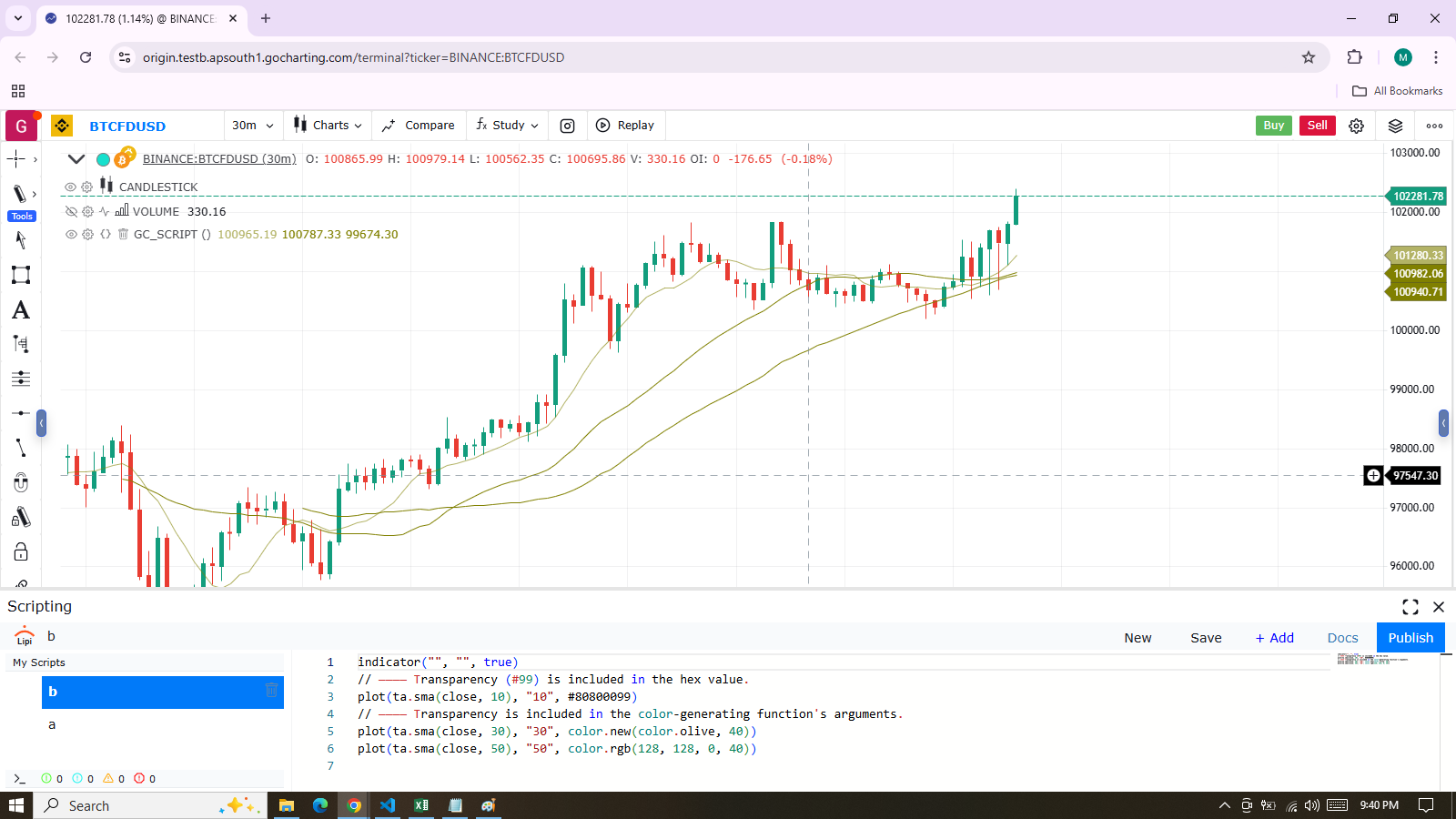
indicator("", "", true)
// ———— Transparency (#99) is included in the hex value.
plot(talib.sma(close, 10), "10", #80800099)
// ———— Transparency is included in the color-generating function's arguments.
plot(talib.sma(close, 30), "30", color.new(color.olive, 40))
plot(talib.sma(close, 50), "50", color.rgb(128, 128, 0, 40))*Notice! The last two
plot()calls use thetranspparameter to specify transparency. This approach should be avoided, as thetranspparameter is deprecated in Lipi Script v5. The use oftranspis less flexible because it requires an input of integer type, meaning the transparency value must be set before the script runs. This prevents it from being calculated dynamically as the script executes on each bar. Additionally, if you provide acolorargument that already includes transparency information (as in the next threeplot()calls), anytranspargument will have no effect. This limitation also applies to other functions that use thetranspparameter.
In the previous script, the colors remain constant as the script runs from bar to bar. However, in some cases, colors need to be created dynamically during execution because they depend on conditions that are not known at compile time or when the script starts running on bar zero. For such scenarios, developers have two options:
- Use conditional statements to select colors from a set of predefined base colors.
- Dynamically generate new colors as the script runs bar by bar, allowing for features like color gradients.
Conditional Coloring
For example, if you want to color a moving average based on specific conditions, you can use a conditional statement to choose a different color for each state. Here’s how you can color the moving average in a “bull” color when it’s rising and a “bear” color when it’s not:
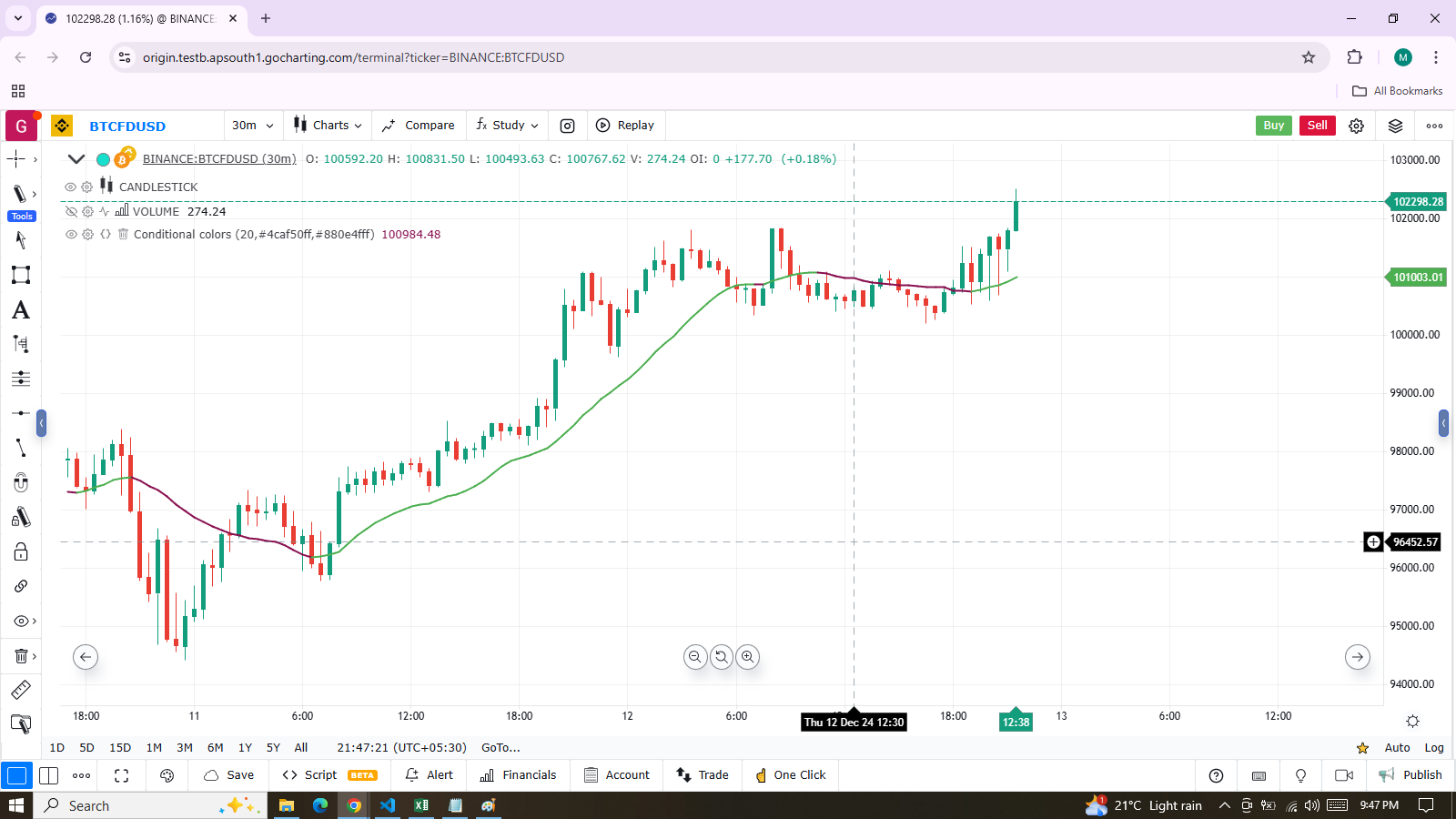
indicator("Conditional colors", "", true)
int   lengthInput = input.int(20, "Length", minval = 2)
color maBullColorInput = input.color(color.green, "Bull")
color maBearColorInput = input.color(color.maroon, "Bear")
float ma = talib.sma(close, lengthInput)
// Define our states.
bool maRising  = talib.rising(ma, 1)
// Build our color.
color c_ma = maRising ? maBullColorInput : maBearColorInput
plot(ma, "MA", c_ma, 2)
Note the following:
- Our script offers users a choice of colors for bull and bear states.
- We create a
maRisingboolean variable that istruewhen the moving average is higher on the current bar compared to the previous one. - A
c_macolor variable is defined, which is assigned one of two colors based on the value of themaRisingboolean. The ternary operator (? :) is used to implement the conditional logic.
Conditional coloring can also be used to prevent plotting under specific conditions. For instance, we plot high and low pivots using a line, but we don’t want to plot anything when a new pivot is detected, to avoid the visual gaps that appear during pivot transitions. To handle this, we check for pivot changes and set the color to na when a change occurs, ensuring that no line is drawn on that bar.
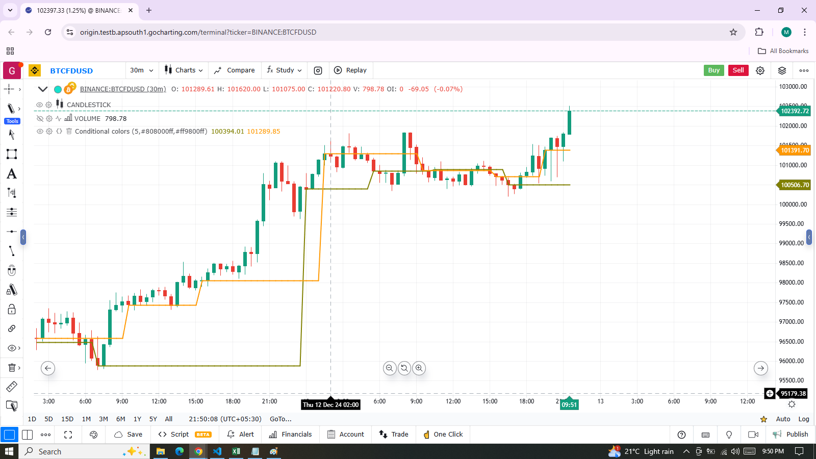
indicator("Conditional colors", "", true)
int legsInput = input.int(5, "Pivot Legs", minval = 1)
color pHiColorInput = input.color(color.olive, "High pivots")
color pLoColorInput = input.color(color.orange, "Low pivots")
// Intialize the pivot level variables.
static float pHi = na
static float pLo = na
// When a new pivot is detected, save its value.
pHi := nz(talib.pivothigh(close, legsInput, legsInput), pHi)
pLo := nz(talib.pivotlow(close, legsInput, legsInput), pLo)
// When a new pivot is detected, do not plot a color.
plot(pHi, "High", talib.change(pHi) ? na : pHiColorInput, 2, plotStyle.line)
plot(pLo, "Low",  talib.change(pLo) ? na : pLoColorInput, 2, plotStyle.line)
Note the following:
- Our script offers users a choice of colors for bull and bear states.
- We create a
maRisingboolean variable that istruewhen the moving average is higher on the current bar compared to the previous one. - A
c_macolor variable is defined, which is assigned one of two colors based on the value of themaRisingboolean. The ternary operator (? :) is used to implement the conditional logic.
To understand how this code functions, it’s important to know that talib.pivothigh() and talib.pivotlow(), when used without an argument for the source parameter, will return a value if a high/low pivot is found. If no pivot is detected, they return na.
When we check the value returned by the pivot function for na using the nz() function, we allow the value to be assigned to the pHi or pLo variables only if it’s not na. If it is na, the previous value of the variable is simply retained, which does not affect its value. Remember that previous values of pHi and pLo are maintained from bar to bar because we use the static keyword during initialization, ensuring that initialization happens only on the first bar.
The final step is to add a ternary conditional statement when plotting the lines. This will return na for the color when the pivot value changes, and use the selected color from the script’s inputs when the pivot level remains the same.
Calculated Colors
By using functions like color.new(), color.rgb(), and color.from_gradient(), you can dynamically generate colors as the script runs from bar to bar.
color.new()is particularly useful when you need to adjust the transparency level of a base color.color.rgb()comes in handy when you need to build colors dynamically by specifying red, green, blue, or transparency components. Additionally, functions likecolor.r(),color.g(),color.b(), andcolor.t()can be used to extract the individual components (red, green, blue, or transparency) of a color, which can then be used to create variants.color.from_gradient()is ideal for creating linear gradients between two base colors. It determines the appropriate intermediary color by evaluating a source value against a minimum and maximum range.
Example with color.new()
Let’s see how color.new(color, transp) can be used to create different levels of transparency for volume columns, using one of two bull/bear base colors:
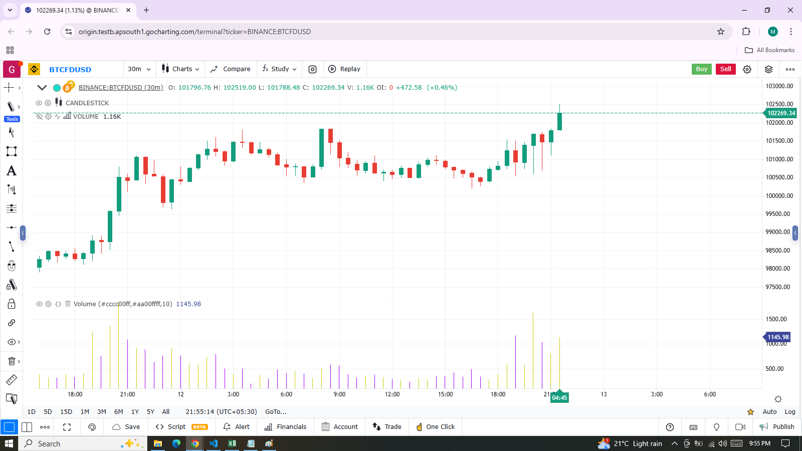
indicator("Volume")
// We name our color constants to make them more readable.
static color GOLD_COLOR   = #CCCC00ff
static color VIOLET_COLOR = #AA00FFff
color bullColorInput = input.color(GOLD_COLOR,   "Bull")
color bearColorInput = input.color(VIOLET_COLOR, "Bear")
int levelsInput = input.int(10, "Gradient levels", minval = 1)
// We initialize only once on bar zero with `static`, otherwise the count would reset to zero on each bar.
static float riseFallCnt = 0
// Count the rises/falls, clamping the range to: 1 to `i_levels`.
riseFallCnt := math.max(1, math.min(levelsInput, riseFallCnt + math.sign(volume - nz(volume[1]))))
// Rescale the count on a scale of 80, reverse it and cap transparency to <80 so that colors remains visible.
float transparency = 80 - math.abs(80 * riseFallCnt / levelsInput)
// Build the correct transparency of either the bull or bear color.
color volumeColor = color.new(close > open ? bullColorInput : bearColorInput, transparency)
plot(volume, "Volume", volumeColor, 1, plotStyle.histogram)
Note the following:
- In the second-to-last line of our script, we dynamically calculate the column color by adjusting both the base color (depending on whether the bar is up or down) and the transparency level. The transparency is calculated based on the cumulative rises or falls in volume.
- The script allows the user to control not only the base bull and bear colors but also the number of brightness levels applied. This value determines the maximum number of volume rises or falls tracked. Giving users the ability to manage this setting allows them to adapt the indicator’s appearance to their specific timeframe or market conditions.
- We ensure that the maximum transparency level never exceeds 80 to maintain some level of color visibility.
- The minimum number of levels is set to 1 in the inputs. When the user selects 1, the volume columns will be displayed in either the bull or bear color at full brightness or with zero transparency.
Using color.rgb()
Creates a new color with transparency using the RGB color model.
Syntax & Overloads
color.rgb(red, green, blue, transp) → const color

example:

```js
//
indicator("color.rgb", overlay=true)
plot(close, color=color.rgb(255, 0, 0, 50))
Another example:
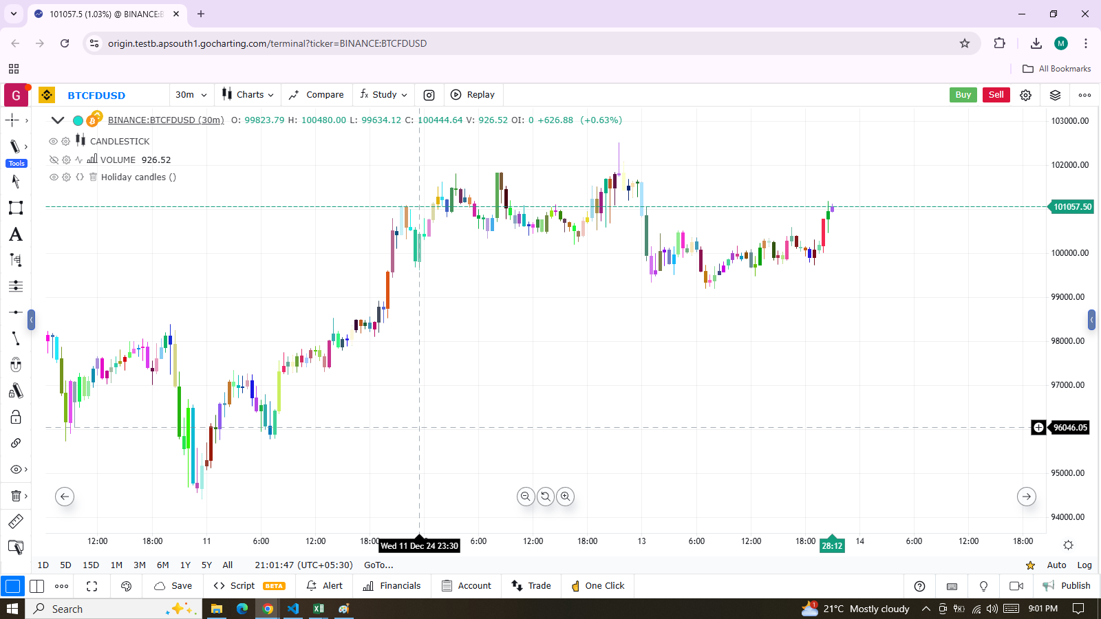
indicator("Holiday candles", "", true)
int r = math.round(math.random(0, 255))
int g = math.round(math.random(0, 255))
int b = math.round(math.random(0, 255))
float t = math.random(0, 1)
color holidayColor = color.rgb(r, g, b, 1)
plotcandle(open, high, low, close, color = holidayColor, wickcolor = holidayColor, bordercolor = holidayColor)
Using color.from_gradient()
The final examples of color calculations will demonstrate the use of color.from_gradient(value, bottom_value, top_value, bottom_color, top_color). First, we will apply it in its simplest form to color a CCI signal in an indicator that otherwise mirrors the built-in version:
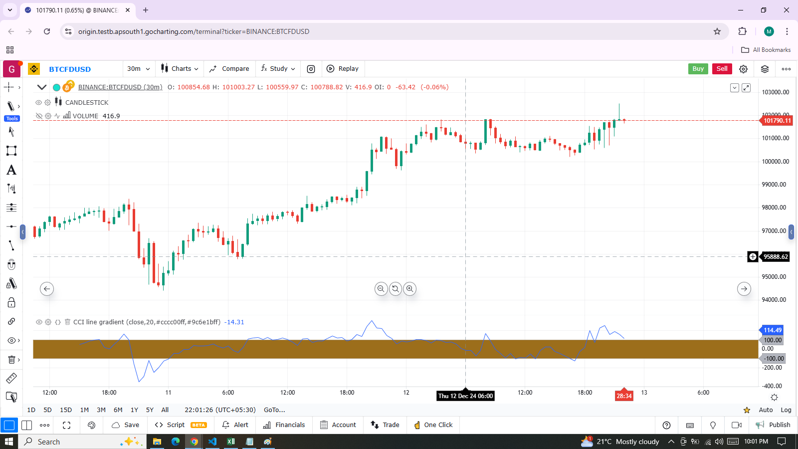
indicator(title="CCI line gradient")
static color GOLD_COLOR = #CCCC00
static color VIOLET_COLOR = #AA00FF
static color BEIGE_COLOR = #9C6E1B
float srcInput = input.source(close, title="Source")
int lenInput = input.int(20, "Length", minval = 5)
color bullColorInput = input.color(GOLD_COLOR,"Bull")
color bearColorInput = input.color(BEIGE_COLOR, "Bear")
float signal = talib.cci(srcInput, lenInput)
color signalColor = color.blue
plot(signal, "CCI", signalColor)
bandTopPlotID = hline(100, "Upper Band", color.silver)
bandBotPlotID = hline(-100, "Lower Band", color.silver)
fill(bandTopPlotID, bandBotPlotID, color = color.new(BEIGE_COLOR, 90), title = "Background")
Note the following:
- To calculate a gradient,
color.from_gradient()requires minimum and maximum values to compare against the argument used for thevalueparameter. While we are working with an unbounded signal like the CCI (which does not have fixed boundaries like RSI, which oscillates between 0-100), this does not prevent us from usingcolor.from_gradient(). In this case, we solve the issue by providing values of -200 and 200 as thebottom_valueandtop_valuearguments. These values do not represent the actual minimum and maximum for CCI but are chosen as thresholds beyond which the colors will no longer change. When the series falls outside thebottom_valueandtop_value, the colors forbottom_colorandtop_colorwill be used. - The color progression generated by
color.from_gradient()is linear. If the series value lies halfway between thebottom_valueandtop_value, the resulting color’s RGBA components will also be halfway between thebottom_colorandtop_color. - Many common indicator calculations are available in Lipi Script as built-in functions. In this case, we use
talib.cci()instead of manually calculating the CCI. - The argument used for the
valueparameter incolor.from_gradient()doesn’t necessarily have to be the value of the line being calculated. Any value can be used, as long as thebottom_valueandtop_valuearguments are provided. For example, in this CCI indicator enhancement, we color the band based on the number of bars since the signal has been above or below the centerline.
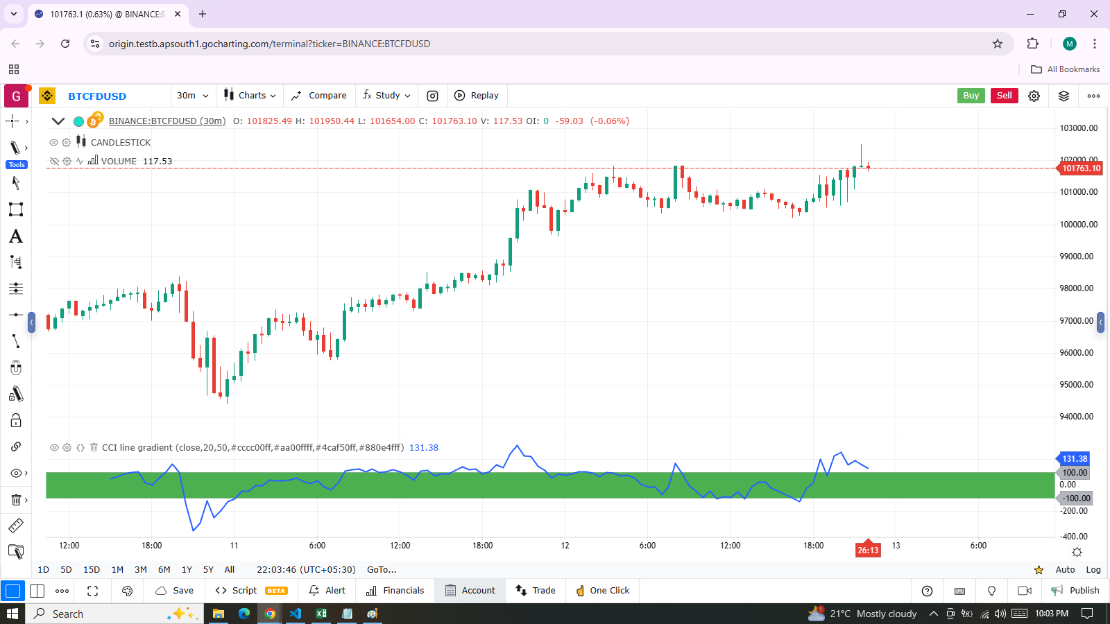
indicator(title="CCI line gradient")
static color GOLD_COLOR   = #CCCC00
static color VIOLET_COLOR = #AA00FF
static color GREEN_BG_COLOR = color.new(color.green, 70)
static color RED_BG_COLOR   = color.new(color.maroon, 70)
float srcInput      = input.source(close, "Source")
int   lenInput      = input.int(20, "Length", minval = 5)
int   stepsInput    = input.int(50, "Gradient levels", minval = 1)
color bullColorInput   = input.color(GOLD_COLOR, "Line: Bull", inline = "11")
color bearColorInput   = input.color(VIOLET_COLOR, "Bear", inline = "11")
color bullBgColorInput = input.color(GREEN_BG_COLOR, "Background: Bull", inline = "12")
color bearBgColorInput = input.color(RED_BG_COLOR, "Bear", inline = "12")

// Plot colored signal line.
float signal = talib.cci(srcInput, lenInput)
color signalColor = color.blue
plot(signal, "CCI", signalColor, 2)

// Detect crosses of the centerline.
bool signalX = talib.cross(signal, 0)
// Count no of bars since cross. Capping it to the no of steps from inputs.
int gradientStep = math.min(stepsInput, nz(talib.barssince(signalX)))
// Choose bull/bear end color for the gradient.
color endColor = signal > 0 ? bullBgColorInput : bearBgColorInput
// Get color from gradient going from no color to `c_endColor`
color bandColor = color.green
bandTopPlotID = hline(100,  "Upper Band", color.silver)
bandBotPlotID = hline(-100, "Lower Band", color.silver)
fill(bandTopPlotID, bandBotPlotID, color = bandColor, title = "Band")
Note the following:
- The signal plot in this example uses the same base colors and gradient as in the previous one. However, we have increased the line width from the default value of 1 to 2. This helps give the signal plot more prominence, ensuring it stands out and doesn’t get overlooked, especially as the band becomes busier than before with its original, flat beige color.
- The fill remains subtle for two main reasons:
- It is of secondary importance to the visuals, serving as complementary information — showing how long the signal has been in bull or bear territory.
- Since fills have a higher z-index than plots, they may cover the signal plot. To avoid this, we reduce the fill’s opacity by setting transparency to 70, ensuring that the plot remains visible beneath the fill.
- The gradient used for the fill starts with no color at all (indicated by
nain thebottom_colorargument of thecolor.from_gradient()function), and gradually transitions to the base bull/bear colors from the inputs, which are contained in thec_endColorconditional variable. - Users are given distinct selections for bull/bear colors for both the line and the band.
- When calculating the
gradientStepvariable, we usenz()ontalib.barssince()because, in the early bars of the dataset, when the condition has not yet been met,talib.barssince()will returnna. Usingnz(), we replace thosenavalues with zero.
Mixing Transparencies
In this example, we further enhance the CCI indicator by building dynamically adjusting extreme zone buffers using a Donchian Channel (DC), which is calculated from the CCI. The top and bottom bands of the DC are set to 1/4 of its height. The lookback period for calculating the DC is adjusted dynamically based on the volatility, which we measure by comparing a short-period ATR to a long-period ATR. If the volatility ratio exceeds 50% of its last 100 values, we consider the volatility to be high, and the lookback is decreased accordingly. Conversely, the lookback is increased when volatility is low.
Our goal is to provide users of the indicator with:
- The CCI line colored using a bull/bear gradient, as shown in previous examples.
- The top and bottom bands of the Donchian Channel, filled with colors that darken over time as historical highs/lows age.
- A visualization of the volatility measure, displayed by painting the background with a color whose intensity increases when volatility is high.
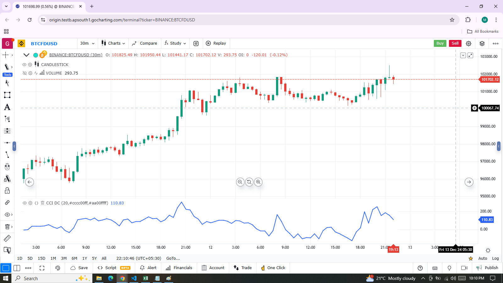
indicator("CCI DC", precision = 6)
color GOLD_COLOR   = #CCCC00ff
color VIOLET_COLOR = #AA00FFff
int lengthInput = input.int(20, "Length", minval = 5)
color bullColorInput = input.color(GOLD_COLOR,   "Bull")
color bearColorInput = input.color(VIOLET_COLOR, "Bear")

// ————— Function clamps `val` between `min` and `max`.
clamp(val, min, max) =>
    math.max(min, math.min(max, val))

// ————— Volatility expressed as 0-100 value.
float v = talib.atr(lengthInput / 5) / talib.atr(lengthInput * 5)
float vPct = talib.percentrank(v, lengthInput * 5)

// ————— Calculate dynamic lookback for DC. It increases/decreases on low/high volatility.
bool highVolatility = vPct > 50
static int lookBackMin = lengthInput * 2
static int lookBackMax = lengthInput * 10
static float lookBack = math.avg(lookBackMin, lookBackMax)
lookBack += highVolatility ? -2 : 2
lookBack := clamp(lookBack, lookBackMin, lookBackMax)

// ————— Dynamic lookback length Donchian channel of signal.
float signal = talib.cci(close, lengthInput)
// `lookBack` is a float; need to cast it to int to be used a length.
float hiTop  = talib.highest(signal, int(lookBack))
float loBot  = talib.lowest( signal, int(lookBack))
// Get margin of 25% of the DC height to build high and low bands.
float margin = (hiTop - loBot) / 4
float hiBot  = hiTop - margin
float loTop  = loBot + margin
// Center of DC.
float center = math.avg(hiTop, loBot)

// ————— Create colors.
color signalColor = color.from_gradient(signal, -200, 200, bearColorInput, bullColorInput)
// Bands: Calculate transparencies so the longer since the hi/lo has changed,
//        the darker the color becomes. Cap highest transparency to 90.
float hiTransp = clamp(100 - (100 * math.max(1, nz(talib.barssince(talib.change(hiTop)) + 1)) / 255), 60, 90)
float loTransp = clamp(100 - (100 * math.max(1, nz(talib.barssince(talib.change(loBot)) + 1)) / 255), 60, 90)
color hiColor = color.new(bullColorInput, hiTransp)
color loColor = color.new(bearColorInput, loTransp)
// Background: Rescale the 0-100 range of `vPct` to 0-25 to create 75-100 transparencies.
color bgColor = color.new(color.gray, 100 - (vPct / 4))

// ————— Plots
// Invisible lines for band fills.
hiTopPlotID = plot(hiTop, color = na)
hiBotPlotID = plot(hiBot, color = na)
loTopPlotID = plot(loTop, color = na)
loBotPlotID = plot(loBot, color = na)
// Plot signal and centerline.
p_signal = plot(signal, "CCI", signalColor, 2)
plot(center, "Centerline", color.silver, 1)

// Fill the bands.
fill(hiTopPlotID, hiBotPlotID, hiColor)
fill(loTopPlotID, loBotPlotID, loColor)

// ————— Background.
bgcolor(bgColor)
Note the following:
- We limit the transparency of the background to a range of 75-100 to ensure it doesn’t overpower the chart. Additionally, we use a neutral color that won’t be too distracting. The darker the background, the higher our volatility measure indicates.
- We also restrict the transparency values for the band fills to between 60 and 90. Using a transparency of 90 ensures that when a new high or low is detected and the gradient resets, the initial transparency will make the color slightly visible. We avoid using transparency lower than 60 to ensure that the bands do not obscure the signal line.
- To generate values that measure volatility, we use the
talib.percentrank()function, which produces a value between 0 and 100 from the ATR ratio. This is useful when converting unknown scale values into known values that can be used to adjust transparencies. - Since we need to clamp values three times in our script, we created an
f_clamp()function to avoid repeating the logic multiple times.
Plot Crisp Lines
For the most important lines in your visuals, it’s best to use zero transparency, which ensures they remain crisp and distinct. These lines will also show through fills more clearly. Note that fills have a higher z-index than plots, so they appear above the lines. A slight increase in the width of a line can also make it stand out more.
If you want a specific plot to be more prominent, consider using multiple plots for the same line. You can modulate the width and transparency of successive plots to achieve this effect:
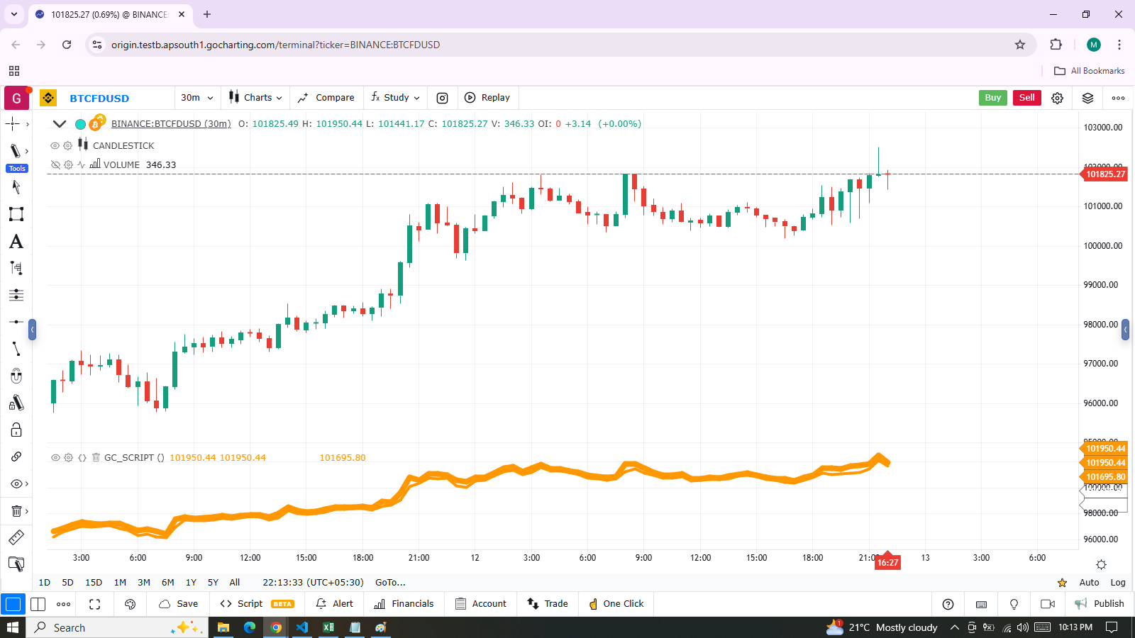
indicator("")
plot(high, "", color.new(color.orange, 80), 8)
plot(high, "", color.new(color.orange, 60), 4)
plot(high, "", color.new(color.orange, 00), 1)

plot(hl2, "", color.new(color.orange, 60), 4)
plot(hl2, "", color.new(color.orange, 00), 1)

plot(low, "", color.new(color.orange, 0), 1)
Customize Gradients
When creating gradients, it’s important to tailor them to the visuals they are applied to. For instance, if you’re using a gradient to color candles, it’s generally best to limit the number of steps in the gradient to ten or fewer. This is because the human eye finds it harder to perceive subtle intensity variations in discrete objects.
As shown in our examples, it’s a good practice to cap the minimum and maximum transparency levels. This ensures your visual elements remain visible, even when transparency is applied, without overwhelming the user when it’s unnecessary.